Nitrous oxide measurements are key to quantifying the photochemical and transport processes that affect Arctic spring ozone

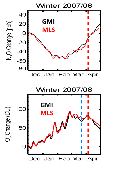
Figure 1: Dashed lines show when the temperature becomes too warm for O₃ depletion (blue) and the vortex breaks down (red).

The Arctic seasonal evolution of simulated Ozone (O₃) and the long lived trace gas Nitrous oxide (N₂O) from the Global Modeling Initiative Chemistry and Transport Model (GMI CTM) both closely agree with MLS observations for all years since Aura's launch in 2004. The northern winter 2008 (Figure 1) is shown as an example. The excellent agreement for N₂O tells us that the model's meteorology is realistic. Because the meteorology is realistic, the good agreement for O₃ tells us that we can accurately quantify the photochemical ozone loss for northern winters 2005 - 2015 using GMI CTM. Ozone's evolution depends on both meteorology and ozone loss.

The Global Modeling Initiative Chemistry and Transport Model (GMI CTM) was run with and without the chemical reactions that cause ozone depletion to quantify the Arctic depletion. We calculated the maximum column O₃ depletion each season averaged over the polar cap (63o-90oN). We also counted the number of days each season that the polar cap temperatures were low enough to form polar stratospheric clouds.

Polar stratospheric clouds (PSCs) play an important role in Antarctic ozone destruction but the extent of PSCs varies a lot from year to year. These high altitude clouds form only at very low temperatures help destroy ozone in two ways: They provide a surface which converts benign forms of chlorine into reactive, ozone-destroying forms, and they remove nitrogen compounds that moderate the destructive impact of chlorine

The maximum O₃ depletion (Figure 2) is a linear function of number of days cold enough to form PSCs. From this we estimate O₃ depletion for the years prior to Aura with similar chlorine levels (1993-2004) using only MERRA temperatures.

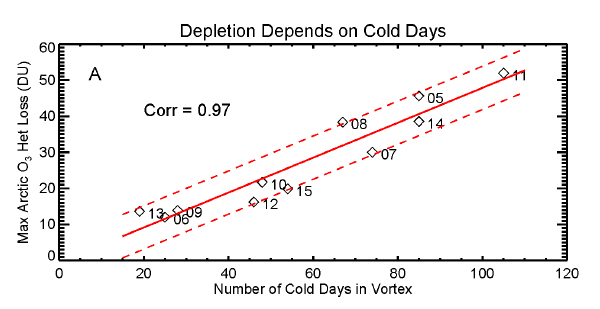
Figure 2: Depletion is a linear function of number of days cold enough to form PSCs.

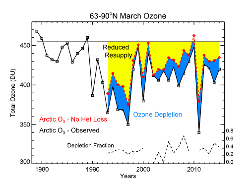
Figure 3 : Patterned after a figure used in WMO Ozone Assessments , this figure shows Arctic spring column O₃ observed by satellites (black), Arctic O₃ depletion calculated in this study (blue shading), and the size of O₃ transport variations each year (yellow).

Significance: Based on the ozone depletion/cold days relationship, we used MERRA temperatures to quantify depletion for years before Aura. The depletion we calculated explains the large interannual variability observed in Arctic March O₃ (figure 3). The horizontal line at 455 DU represents the assumed 'undepleted' level of Arctic spring O₃.

We found that ~2/3 of the observed interannual variability (figure 3/yellow) was caused by variations in the O₃ transported to the polar region while only ~1/3 was due to depletion (figure 3/blue). Both of these variations are controlled by the strength of wave energy entering the Arctic stratosphere each winter. More wave energy means higher Arctic O₃. The greatest Arctic ozone depletion (63-90°N average) in this period was 10% and it occurred in 2011.

Relevance for Future Science: MLS N₂O and O₃ measurements and the GMI chemistry transport model integrated with meteorological reanalyses provide a means to understand how chemistry and transport work together when polar ozone changes. The model and data combination make it possible the attribute the causes of O₃ variations. Attribution is critical for identifying ozone recovery due to the Montreal Protocol. No other satellite, ground-based, or aircraft instruments provide daily global dynamical and chemical information comparable to MLS .

Data Sources: Aura Microwave Limb Sounder O₃ and N₂O version 4; the NASA MERRA reanalysis.

References: Strahan, S. E., A.R. Douglass, S.D. Steenrod (2016), Chemical and Dynamical Impacts of Stratospheric Sudden Warmings on Arctic Ozone Variability, J. Geophys. Res., 121, 11,836-11,851, doi:10.1002/2016JD025128.

2.07.2017